Re-visiting climate forcing/feedback concepts…

I haven’t been able to post much lately, so I just want to put in this post which outlines some of the basic radiative forcing and feedback physics which climatologists use to assess climate change. This is fairly standard material which should be understood by anyone with a deep interest in climate. This article is a bit lengthy so hopefully you have the patience to go through it (or put it on your favorites and come back). Also, a lot of discussion has come up recently over Richard Lindzen’s ERBE analysis in which he purports to show that global climate sensitivity is small, and that the net effect of climate feedbacks is to dampen the so-called Planck response. That basically provoked this post. I’m going to define all these terms below, so don’t worry if I’ve already lost you, and while I am going to do some math in this post, it should be accessible to most people who know a bit of algebra. Skipping over a few calculus steps won’t be detrimental and I’ve tried not to assume much climate background (although I do link to some side references for clarification on some matters). My focus is not on Lindzen’s analysis here, which I don’t feel to be robust at all, but rather building up simple mathematical models for understanding climate change. This will not be new to anyone who has followed the climate literature or discussions for some time, but hopefully it can be helpful to some, or at the very least, serve as a useful reference.

The primary focus of study within the atmospheric sciences for grasping how climate change works is in electromagnetic radiation, and how radiative fluxes interact with the surface and atmosphere interface. We can keep this simple and imagine that planets take in light only at short wavelengths of the EM spectrum from the sun (mostly in the visible region), and that planets emit light back to space only in the longer wavelengths, in the thermal infrared part of the spectrum. As seen below, we can distinguish easily between the solar radiation curves and terrestrial radiation curves, which hardly overlap at all across roughly the 4 micron threshold:

For all the terrestrial planets (Venus, Mars, Earth) we can say that the heating due to radioactive decay in the Earth’s interior is negligible, and they only gain and lose heat radiatively (since outer space is a vacuum).

The radiative balance at the top of the atmosphere acts as the fundamental boundary condition which constrains the global climate. In this model, we assume that the energy input by the sun at the top of Earth’s atmosphere ends up being balanced by the outgoing infrared radiation to space. This is true over sufficiently long timescales when the climate is not undergoing change. If it were not true, then the planet would either warm or cool depending on whether more energy was coming in than going out, or more was going out than coming in. The simplest model for radiative balance can then be written as:

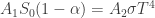
The “A” terms describe the area of which the planet receives or emits radiation. For Earth, the outgoing energy leaves in all directions, so we can take the area to be however, the incoming energy only comes in like a circle (essentially the shadow that would be cast by the planet) because the sunlight comes in from just one side and is not as intense over the whole half-sphere. Thus the A₁ term is . In reality, the ratio of A₂ to A₁ is about 4.0034 (Loeb et al 2009) and not 4, since the Earth is not a perfect sphere, but the algebra is made much easier in assuming sphericity, and the radius of the Earth becomes irrelevant since those terms cancel out. S₀ here is the solar constant, which is the radiative flux (in Watts per Square meter) that would be intercepted by a flat “wall” in space which stood perpendicular to the incoming solar rays. For a planet at the mean Earth-sun distance, the solar constant is about 1370 W/m². is thus the incoming solar radiation averaged over the spherical Earth, with a factor of at the equator and declining like the cosine of the latitude angle as you move toward the poles. is the albedo of the planet, which is the fraction of incoming solar radiation that is reflected right back out to space (mostly clouds, but also by various land surfaces, brighter ones like ice or desert sand contributing strongly). The fraction of absorbed sunlight is therefore 1- . The albedo of the Earth is presently about 0.3 (i.e., 30% of the incoming solar energy is reflected back to space). is the Stefan-Boltzmann law which relates the total power output (per unit area) of a body to a given temperature, and sigma is about 5.67 * 10^-8 W/m²/K⁴. Basically it shows that hotter bodies radiate much more than cooler bodies, because of the strong fourth power dependence. Temperatures must be expressed in Kelvins. From all this, we can solve for an “effective temperature” of a hypothetical planet which essentially radiated like a perfect blackbody and had uniform temperature over the globe:

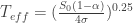
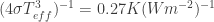
Plugging in all the relevant parameters into the equation, the effective temperature becomes about 255 K, or about 0 degrees F. The reason why the planet is not actually this cold is because the atmosphere acts to inhibit the efficiency at which the outgoing infrared radiation escapes to space. This is the greenhouse effect, and is caused by molecules (water vapor, CO2, ozone, methane, mostly) which strongly interact with infrared radiation at Earth-like conditions. I’ve already done a couple of posts (see updated this post) on how the greenhouse effect works, and I’m assuming most readers are either educated in that or can get a somewhat decent understanding by reading the above links (wiki actually does a good job IMO). These will also help place the preceding discussion in better context.

We’ve already established that at equilibrium, the difference between the absorbed sunlight and outgoing energy at the top of the atmosphere is zero. Now suppose we perturb the climate system and force the global temperature to change by changing the amount of sunlight we get (or the planetary reflectivity), or as is the case in modern times, changing the outgoing infrared radiation with greenhouse gases. We quantify such a perturbation in terms of radiative forcing, or loosely the difference between the incoming radiation energy and the outgoing radiation energy (there’s some caveats in here about allowing the stratosphere to adjust to equilibrium, and some people define forcing at the tropopause or Top Of Atmosphere, and other alternate definitions have come up in the primary literature, but those details are not really important right now).

We can include a number of different forcings which may have competing effects (e.g., greenhouse gas increase would warm the planet, turning down the sun would cool, increasing sulfate-based aerosols would raise the albedo and cool the planet a bit). We can also introduce an efficacy factor (described in Hansen et al 2005) which is the global temperature response per unit forcing for a given forcing agent relative to the response to a standard CO2 increase,

Where FA is the climate forcing, and the summation includes all relevant radiative forcings over a certain time period. Efficacy arises because not all forcings produce the same relative impact, and some produce stronger or weaker changes in climate than CO2 (defined so = 1) for the same forcing. The radiative forcing for CO2 (as described in Myhre et al 1998 and later papers) is

Where the constant k (derived from line-by-line radiative transfer codes) is typically taken to be 5.35 W/m², and C and C₀ are the final and initial CO2 concentrations. Using this simple relation results in a forcing of nearly 4 W/m² for each doubling of CO2. Note that the logarithmic relation suggests that the fractional change in CO2 is what is important, since every doubling produces the same effect. In that sense, adding 10 ppmv of CO2 to a background concentration of 20 ppmv would produce a much larger change than adding 10 ppm to a background concentration of 1000 ppmv. This relation holds well over relevant Earth-like conditions, however the forcing becomes stronger than logarithmic at very low or very high concentrations. Also note this is the forcing at the tropopause, not the surface. Here is a table of modern day forcings relative to 1750 values (IPCC 2007)

It makes sense to ask now what this actually means for us. In other words, how much temperature rise would you get for a given forcing? We use a matric called climate sensitivity to make sense of this. Climate sensitivity is the temperature response of the system per unit forcing. In other words, a high climate sensitivity means that it is very easy to change the global mean temperature, while a very low sensitivity would require an enormous forcing to get that same change. In the easiest case, we’ll consider what happens when you only increase some forcing (say double CO2) and allow the outgoing radiation to increase (according to the Stefan-Boltzmann law) to re-establish a new radiative equilibrium. Here, nothing else changes with the climate state (no cloud cover changes, no ice melts, etc) except for our forcing. This is the so-called Planck response. In a simple way, we can assume that the surface and emission temperature are linearly related, in which case the Planck-only feedback response can be computed as the inverse of the derivative of Stefan-Boltzmann with respect to temperature,

Which equals,

The temperature response can then be linearly related to a forcing

Where is the Planck-feedback factor described above. It is important to note now that this is an equilibrium formula, meaning that we don’t see the full temperature response to show up right away if we instantly double CO2, since it takes time for the radiative imbalance to go to zero (it’s hard to heat up the oceans quickly!). We’ll see that when we actually allow other things like clouds,water vapor, albedo, etc to vary with the climate response (as opposed to the unrealistic stefan-boltzmann only feedback), then lambda becomes a function of all those things, and describes how the total forcing is connected to the temperature response. This formula implies that for a 4 Watt per square meter forcing (remember, about a doubling of CO2 equivalent), you get roughly a 1 K temperature rise (multiply these numbers by two to get changes in Fahrenheit).

To compute a radiative forcing for an increase in solar irradiance, we do

where the 1/4 and 0.7 factor account for the geometry and albedo of the Earth, respectively. Depending on how radiative forcing is defined, this number can often be reduced further to account for ozone absorption of UV or other effects, but in general the forcing due to a realistic change in solar increase is very small. It follows that it would take about a 22 W/m² change in solar irradiance to produce a 1 K change in global temperature. This is actually a very stable climate. This also demonstrates the intellectual bankruptcy of those who claim that the solar trend over the last half century (which has pretty much been a flat-line when you remove the 11-year oscillatory signal) is responsible for most of the observed late 20th century warming, and simultaneously argue for a low sensitivity.

Paleoclimate evidence suggests much larger climate changes have occurred than is possible under realistic forcing scenarios given this sort of sensitivity. The magnitude of glacial-interglacial cycles for instance is on the order of 4-6 K in the global mean, and when you go back in time far enough, much larger climate changes are possible. Even observed trends over the 20th century do not appear to be compatible with a very small sensitivity factor. A useful summary of Earth’s equilibrium sensitivity evidence can be found in Knutti and Hegerl 2008. The best available evidence over the last few decades of research (discussed in IPCC 2007 especially) hints at an equilibrium temperature sensitivity of 2 to 4.5 K (as opposed to 1 K) per doubling of CO2. It can thus be inferred (and supported by a larger body of evidence) that other things are acting to amplify the Planck-response to create a climate which is more sensitive to changes. This will be elaborated upon briefly.

The 2 to 4.5 K value range is the so-called Charney sensitivity. Remember this is the equilibrium response, not the immediate response, and so this is probably not a realistic realization for what to expect over the course of this century. The transient response for a doubling of CO2 (this is defined by assuming that CO2 increases by 1% per year and then recording the temperature increase at the time CO2 doubles) is about 1.3 to 2.6 K in the CMIP3 archive (USCCP 2008) which is less than the longer-term response, and also features less uncertainty. There is also a very long climate sensitivity response which is relevant on timescales of many hundreds to thousands of years and included “slow feedbacks” like ice sheet changes, and is on the order of around 5 K for a doubling of CO2.

Now we consider feedbacks to understand why the actual climate response differs so much from what you’d expect with just the radiative forcing and radiative adjustment. A feedback is essentially something which acts to amplify or dampen the initial forcing. The important distinction is that the forcing “pushes” the climate into a new state, and the feedback simply responds (it doesn’t occur on its own in a stable climate), either pushing the system further in the direction of the initial forcing (positive feedback) or dampening the response which brings the system closer to the initial climate state (negative feedback). The primary radiative feedbacks are water vapor feedback, the lapse rate feedback, cloud feedbacks, and surface albedo feedbacks. Useful summaries of this science can be found in Bony et al 2006 for example, although there’s a lot of good literature here. IPCC 2007 is generally the most comprehensive. I’ll briefly summarize the individual feedbacks below. We now see that lambda is not the Planck-feedback value, but instead is a function of all the possible feedbacks which can occur, and is thus different than the no-feedback scenario (unless all the possible feedbacks happened to cancel out perfectly)

Where these things can also be separated into longwave and shortwave radiation components. Note that the Earth is very inefficient at reflecting infrared radiation at all, so this is not an important term. Reflection of visible radiation is very important however as we’ve seen in describing albedo. Gases in the atmosphere are generally not very good at absorbing incoming sunlight, but rather make the atmosphere opaque to the outgoing infrared. If we change some external variable (e.g., solar constant, more CO2), which we’ll call , and the response depends on a number of other variables, x_j (which are then related to ), then

where the summation ranges from j=1 to the number of important response variables, which could be large, with each component having different (or sometimes self-competing) effects that complicates the picture. Indeed, future projection for climate change to a given change in CO2 is much more uncertain in then it is in the forcing, since GHG forcing uncertainties are typically very small. Aerosol forcings are more uncertain (and restrict knowledge of the total 20th century forcing) but GHG changes should strongly outweigh aerosol changes over the 21st century. Accordingly, future prediction of temperature change depends very much on understanding the individual response variables to climate change and the total response. The following descriptions are far from sufficient, but just to get the feet wet

Water Vapor:

The saturation vapor pressure of water (loosely, “the amount of water the air can hold”) increases nearly exponentially with temperature. This follows from the Clausius-Clapeyron equation (Pierrehumbert et al 2007):

Where TR and are a reference temperature and saturation pressure (614 Pa at 273 K) and x corresponds to the latent heat of the phase transition divided by the gas constant, and takes a value of 5419 K for condensation into liquid and 6148 K for condensation into ice. The dominant influence of the saturation vapor pressure is temperature, increasing sharply, with a 3 K temperature resulting in roughly 20% change in saturation pressure. However, the radiative influence of water vapor depends on the fractional change of water vapor (just like CO2) and not the absolute increase, and so the absorptivity goes as the logarithm of the vapor mass change. Note that this has nothing to do with relative humidity (the fraction of vapor held in air to its saturation amount), but rather specific humidity. Why relative humidity is often discussed in water vapor feedback context is to see how the actual water vapor change scales with the upper limit provided by Clausius-Clapeyron. In the global mean, RH tends to remain roughly constant, which coupled with a change in temperature will yield a positive feedback.

The effect of water vapor is to reduce the outgoing radiation vs. temperature curve, effectively making the climate much more sensitive to forcing. It is important to note that most of the water vapor feedback occurs in the higher altitudes where it is dry and temperatures are cold, and so can be most effective at reducing the outgoing radiation to space. It is also most important in the tropics. The lower level boundary layer water vapor has relatively little to do with water vapor feedback (although it does have implications for other hydrological responses to climate change). Furthermore, water vapor also absorbs visible radiation. This component is far less important than the infrared part, although it can be important in the polar regions where you have scattering from a high surface albedo.

Observations and models are in basic agreement that the upper troposphere becomes moister in a warming climate (e.g., Soden et al 2005), global relative humidity is approximately conserved, and thus enhancing the warming. A good summary of water vapor feedback science that is up-to-date is the Dessler and Sherwood 2009 perspective piece in Science. Water Vapor feedback is the most powerful positive feedback and enhances the warming forced by CO2 by a factor of roughly two.

Lapse Rate:

Because the greenhouse effect depends on the temperature decline with height, decoupling the atmosphere from its current vertical temperature structure will also change the surface temperature. As it is, the whole troposphere is pretty much created by convection, and when it warms or cools it does so as a unit in a way that keeps it near a moist adiabatic lapse rate. The lapse rate change tends to offset some of (but not all) the water vapor feedback. Counterbalancing the water vapor feedback results in warmer temperatures at the high altitudes, more water vapor meaning more condensation, and lifting to higher altitudes so that any given layer of the atmosphere is now radiating more efficiently to space. This can be seen in a simple diagram which shows a steepening of the moist adiabat curves as the climate warms. It follows that “moist regions” will tend to be amplified at altitude relative to the surface.

See here for a larger version of this diagram. The lapse rate feedback tends to thus be negative in regions of moist convection at the tropics, but positive in the high latitudes where surface warming is expected to be amplified. The net effect globally is a negative feedback. This issue also surrounds the whole “hotspot” argument that I’ve discussed before, and whether or not the low-latitude troposphere actually has been amplified relative to the surface. Note again that the hotspot is not a manifestation of higher CO2, just higher temperatures and the fact that we see a moist adiabatic structure during El Nino, the solar cycle, etc. In reality, if such a hotspot doesn’t exist, it just means a less negative lapse rate feedback.

Surface Albedo:

Because the reflectivity of the planet is so important (see Equation. 1) since it directly relates to the absorbed solar energy, changes in the surface that accompany climate change will act as feedback. This occurs when the ratio of a high albedo surface to a low albedo surface increases or decreases in time. The best example is with sea ice, since ice extent tends to increase (decrease) in a cooling (warming) planet, and since ice is much more reflective than surrounding ocean or land, you get a positive feedback. This is one large component of “polar amplification” which describes why high latitudes are more sensitive to climate change than lower latitudes. Warm (cold) climates are therefore characterized by weak (strong) pole-to-equator temperature gradients. Less ice in a global warming situation means more solar absorption which winds up resulting in higher surface air temperatures. The same idea applies to a once forested area which becomes a desert. Sea ice is included in the Charney sensitivity, but not long-term changes in the much larger ice sheets.

It is a very robust result seen in observations and universally across models that the Arctic will warm faster than the Northern Hemisphere as a whole. Over anthropogenic timescales, the Northern amplification is also much more pronounced than at the South Pole. A somewhat more complete picture is that as the climate warms, the summer melt season lengthens which results in reduced sea ice at summer’s end. The summertime absorption of solar radiation in open areas enhances the sensible heat content of the ocean, and thus ice formation in the autumn and winter is delayed. Note that the surface is not highly amplified in the summer where excess energy goes into evaporation or melt, but enhanced upward heat fluxes in the cooler months result in increased temperatures in the lower atmosphere.

Clouds:

Clouds are the largest source of uncertainty in quantifying the extent of climate feedbacks. I’m not actually going to talk about them here (maybe soon! I’d like to explore the various hypotheses and evidence in much better detail) but suffice to say that clouds have competing effects between reflecting sunlight (low clouds mostly) and influencing the outgoing infrared radiation (high clouds mostly). It is still not clear how these two effects will balance out, and thus the magnitude and even the sign of the feedback is not well constrained. It’s probably not very big in either direction, although much of the uncertainty range in the 2 to 4.5 K values for a doubling of CO2 is because we just don’t have clouds nailed down yet in a satisfactory manner. Cloud influence also depends on latitude, optical thickness, and a host of other issues.

Feedbacks behave in a power series like fashion, with small and diminishing gains as time progresses. This looks like g + g² + g³… and so forth, so the temperature response can be related to the planck-only response and the gain factor as

Here, “the sum of g’s” must be less than unity to allow for the possibility of positive feedbacks while still not allowing a “runaway” effect that is unstable. Note also that the feedbacks operate dependently on each other, so a stronger water vapor feedback would mean warmer temperatures, still less ice, a still lower albedo, and so forth.

Below is a plot showing relative strengths of individual feedbacks for water vapor, water vapor+lapse rate, albedo, CRF (not discussed), and clouds, computed for 14 coupled ocean–atmosphere models.

_{Soden et al 2008}

References:

_{Bony, S., R. Colman, V.M. Kattsov, R.P. Allan, C.S. Bretherton, J.-L. Dufresne, A. Hall, S. Hallegatte, M.M. Holland, W. Ingram, D.A. Randall, D.J. Soden, G. Tselioudis, and M.J. Webb, 2006: How well do we understand and evaluate climate change feedback processes? J. Climate, 19, 3445-3482, doi:10.1175/JCLI3819.1}

_{CCSP, 2008: Climate Models: An Assessment of Strengths and Limitations. A Report by the U.S. Climate Change Science Program and the Subcommittee on Global Change Research [Bader D.C., C. Covey, W.J. Gutowski Jr., I.M. Held, K.E. Kunkel, R.L. Miller, R.T. Tokmakian and M.H. Zhang (Authors)]. Department of Energy, Office of Biological and Environmental Research, Washington, D.C., USA}

_{Dessler, A.E., and Sherwood, S.C. A matter of humidity, Science, 323, 1020-1021, DOI: 10.1126/science.1171264, 2009.}

_{Forster, P., V. Ramaswamy, P. Artaxo, T. Berntsen, R. Betts, D.W. Fahey, J. Haywood, J. Lean, D.C. Lowe, G. Myhre, J. Nganga, R. Prinn, G. Raga, M. Schulz and R. Van Dorland, 2007: Changes in Atmospheric Constituents and in Radiative Forcing. In: Climate Change 2007: The Physical Science Basis. Contribution of Working Group I to the Fourth Assessment Report of the Intergovernmental Panel on Climate Change [Solomon, S., D. Qin, M. Manning, Z. Chen, M. Marquis, K.B. Averyt, M.Tignor and H.L. Miller (eds.)]. Cambridge University Press, Cambridge, United Kingdom and New York, NY, USA.}

_{Hansen, J., Mki. Sato, R. Ruedy, L. Nazarenko, A. Lacis, G.A. Schmidt, G. Russell, I. Aleinov, M. Bauer, S. Bauer, N. Bell, B. Cairns, V. Canuto, M. Chandler, Y. Cheng, A. Del Genio, G. Faluvegi, E. Fleming, A. Friend, T. Hall, C. Jackman, M. Kelley, N.Y. Kiang, D. Koch, J. Lean, J. Lerner, K. Lo, S. Menon, R.L. Miller, P. Minnis, T. Novakov, V. Oinas, Ja. Perlwitz, Ju. Perlwitz, D. Rind, A. Romanou, D. Shindell, P. Stone, S. Sun, N. Tausnev, D. Thresher, B. Wielicki, T. Wong, M. Yao, and S. Zhang, 2005: Efficacy of climate forcings. J. Geophys. Res., 110, D18104, doi:10.1029/2005JD005776}

_{Knutti, R. and G. C. Hegerl, 2008, The equilibrium sensitivity of the Earth’s temperature to radiation changes, Nature Geoscience, 1, 735-743, doi:10.1038/ngeo337}

_{Loeb, N.G., B.A. Wielicki, D.R. Doelling, G.L. Smith, D.F. Keyes, S. Kato, N. Manalo-Smith, and T. Wong, 2009: Toward Optimal Closure of the Earth’s Top-of-Atmosphere Radiation Budget. J. Climate, 22, 748–766}

_{Myhre, G., E. J. Highwood, K. P. Shine, and F. Stordal., 1998. New estimates of radiative forcing due to well-mixed greenhouse gases. Geophysical Research Letters, 25, 2715–2718}

_{Pierrehumbert RT, Brogniez H, and Roca R 2007: On the relative humidity of the atmosphere. in The Global Circulation of the Atmosphere, T Schneider and A Sobel, eds. Princeton University Press}

_{Soden, B. J., D. L. Jackson, V. Ramaswamy, M. D. Schwarzkopf, and X. Huang, 2005: The radiative signature of upper tropospheric moistening. Science, 310(5749), 841-844}

_{Soden, B.J., I.M. Held, R. Colman, K.M. Shell, J.T. Kiehl, and C.A. Shields, 2008: Quantifying climate feedbacks using radiative kernels. Journal of Climate, 21, 3504-3520}